

 English
 русский
 Español
 عربى

No. 8, Duxiu San Road, Ganlin Town, Shengzhou City, Shaoxing City, Zhejiang Province, China

News Category
Product Category
Back EMF of a BLDC Motor: How to Calculate It From Speed, Kv, and Flux
Content
- 1 The Core Formula and What Each Symbol Means
- 2 Converting Kv, Ke, and Datasheet Units Without Costly Mistakes
- 3 Calculating From Physical Dimensions and Flux Linkage
- 4 Measurement Method: Scope, Drill, and a Safe No-Load Spin
- 5 Why the Terminal Voltage Is Not the Back EMF Under Load
- 6 Putting the Calculation Into a Motor Enquiry
- 7 Worked Examples and a Final Sanity Check
A 48 V BLDC fan motor is running at 3,000 rpm, and the oscilloscope shows a 30 V peak line-to-line waveform. The controller’s sensorless zero-crossing threshold is set near half the DC bus. Will the motor start reliably, and is the measured voltage actually the back EMF? The answer depends on how the back EMF constant is defined, whether the value is phase or line-to-line, and whether it is peak or RMS. Getting those definitions wrong can turn a simple calculation into a wrong controller setting or a mismatched motor order.
The short answer is: calculate back EMF from E = Ke × ω, where Ke is the back EMF constant and ω is mechanical angular speed. Use the same phase/line and peak/RMS basis as the constant. If only Kv is available, convert it first. If the motor is already on the bench, measure the waveform and calculate Ke from a known speed. The sections below show each method, the unit conversions that cause most errors, and the checks worth doing before a purchase order is released.
The Core Formula and What Each Symbol Means
For a first-pass calculation, use the mechanical form:
Ephase,peak = Kephase,peak × ωm
Here, ωm is shaft speed in radians per second: ωm = 2πn / 60, with n in rpm. Ke must be in V per rad/s. If the datasheet gives Ke in V/krpm, V/rpm, or Kv in rpm/V, convert it before multiplying. The same equation works for a trapezoidal BLDC motor and a sinusoidal PM machine, but the waveform interpretation changes: for trapezoidal motors, use the flat-top amplitude; for sinusoidal motors, use peak or RMS consistently.
For a sinusoidal machine with known flux linkage, the physical form is:
Ephase,peak = p × λm × ωm
where p is the number of pole pairs and λm is the peak flux linkage per phase in Wb-turns. The RMS phase value is Ephase,peak / √2. For line-to-line sinusoidal voltage, multiply the phase RMS value by √3. For a six-step trapezoidal motor, the line-to-line flat top is often close to twice the phase flat-top value, but confirm the waveform because the exact relationship depends on commutation and winding arrangement.
| Quantity | Symbol | Unit | What to confirm |
|---|---|---|---|
| Mechanical speed | n | rpm | Shaft speed, not electrical frequency |
| Angular speed | ωm | rad/s | ωm = 2πn / 60 |
| Back EMF constant | Ke | V/(rad/s) | Phase or line-to-line; peak or RMS |
| Phase back EMF | Eph | V | Use the same basis as Ke |
| Line-to-line back EMF | ELL | V | √3 for sinusoidal RMS; about 2× flat top for trapezoidal |
| Electrical frequency | fe | Hz | fe = p × n / 60 |
Converting Kv, Ke, and Datasheet Units Without Costly Mistakes
Kv is usually stated in rpm per volt. For a no-load DC-style calculation, the back EMF constant in V/(rad/s) is:
Ke = 60 / (2π × Kv) = 9.549 / Kv
If Kv is 100 rpm/V, Ke is about 0.0955 V/(rad/s). At 3,000 rpm, ωm is 314.16 rad/s, so the calculated back EMF is about 30.0 V. If the datasheet defines Kv on a line-to-line basis, that 30.0 V is a line-to-line value. If Kv is phase-based, it is a phase value. The number is the same only when the basis is the same.
For industrial motors, Ke is often given in V/krpm. Convert it by dividing by 104.72, because 1,000 rpm equals 104.72 rad/s. A Ke of 12 V/krpm is therefore 0.1146 V/(rad/s). At 1,500 rpm, the back EMF is 0.1146 × 157.08 = 18.0 V on the same phase/line basis as the datasheet.
A common purchasing risk is a supplier quoting “Ke = 0.12” without units. Is that V/rpm, V/(rad/s), V/krpm, phase peak, or line-to-line RMS? A factor of 2 or √3 can be hidden in that single number. Ask for the definition in writing, and ask for the waveform and test speed used to obtain it. If the motor is intended for sensorless control, also ask for the back EMF at the minimum operating speed, not only at rated speed.
Calculating From Physical Dimensions and Flux Linkage
When a prototype has no useful datasheet, flux linkage is the most direct route. If the design team knows the peak flux linkage per phase, use Ephase,peak = p × λm × ωm. For example, p = 4, λm = 0.05 Wb-turns, and n = 1,500 rpm gives ωm = 157.08 rad/s. The peak phase back EMF is 4 × 0.05 × 157.08 = 31.4 V. The RMS phase value is 22.2 V, and the sinusoidal line-to-line RMS value is 38.5 V.
If flux linkage is not available but the winding and magnetic circuit are known, the calculation can be built from turns per phase, winding factor, air-gap flux per pole, and speed. In practice, the uncertainty in air-gap flux density, lamination stacking factor, and end-winding effects is large enough that a calculated value should be treated as a design estimate. Wind a sample, spin it at a safe speed, and measure the waveform. That measurement is also the fastest way to confirm whether the intended waveform is closer to sinusoidal or trapezoidal. For background on commutation and waveform behavior, the BLDC working-principle article is a useful reference.
Measurement Method: Scope, Drill, and a Safe No-Load Spin
On the bench, disconnect the controller and spin the motor with a drill, a lathe, or another motor. Measure line-to-line voltage with a differential probe or an isolated oscilloscope input. Do not exceed the probe’s common-mode rating, and do not connect a grounded oscilloscope probe to a live three-phase bridge. At a known speed, capture the waveform and record either the flat-top amplitude or the sinusoidal peak and RMS values, depending on the motor type.
Calculate Ke from the measured voltage and speed: Ke = Emeasured / ωm. Then verify electrical frequency with fe = p × n / 60. A four-pole-pair motor spinning at 1,200 rpm should show 80 Hz electrical frequency, or a 12.5 ms period. If the frequency is wrong, check the pole count or the actual shaft speed. If the amplitude is lower than expected, check probe attenuation, winding connection, and whether the measurement is phase or line-to-line.
For a quick production check, spin at a low fixed speed, record the peak-to-peak line voltage, and compare it with a known-good sample. This does not replace a full motor test, but it catches wrong winding turns, reversed phases, and magnet problems before the motor reaches the assembly line. Keep the test speed well below the maximum rated speed and use a guarded test fixture.
Why the Terminal Voltage Is Not the Back EMF Under Load
At no load, terminal voltage is close to back EMF because the current is small. Under load, the applied voltage must overcome back EMF, resistive drop, and inductive drop: Vphase = Ephase + I × R + L × di/dt. A motor with 0.5 Ω phase resistance carrying 10 A has a 5 V resistive drop before any inductance or inverter loss is considered. That is why a calculation made from the DC bus alone can overstate the available speed or underestimate the current at a given load.
PWM operation adds another layer. The inverter applies a chopped voltage, and the motor current ripple depends on switching frequency and inductance. Diode drops, dead time, and cable resistance also remove voltage margin. For sensorless control, the zero-crossing comparator sees the terminal waveform, not an ideal back EMF source. Filters used to remove PWM noise introduce phase delay, and the delay becomes more important as electrical frequency rises. Calculate the expected back EMF at the minimum and maximum speeds, then check the comparator threshold and filter delay against those values.
Putting the Calculation Into a Motor Enquiry
A useful enquiry states the required back EMF at a defined speed, the DC bus range, the phase/line basis, and the acceptable tolerance. For example: “At 2,400 rpm, line-to-line peak back EMF must be 42 V ±5%, measured with the motor at 25 °C and driven by an external prime mover.” That is much clearer than asking for a “0.2 Ke motor” because it removes the unit ambiguity before samples are built. If the motor is for a fan or air-cooler application, also state the load curve and the minimum speed at which sensorless starting must work.
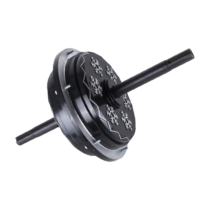
For air-cooler duty, an external-rotor BLDC motor can simplify the mechanical package because the fan can mount directly to the rotor. A representative option is the 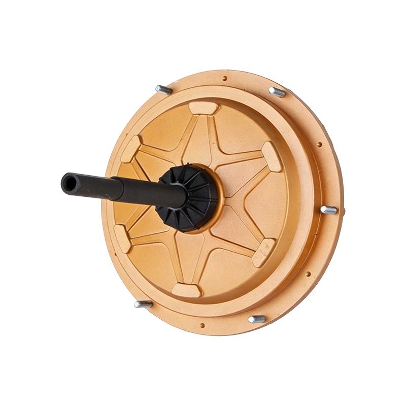 DC149 220V 600W External BLDC Air Cooler MotorExternal-rotor 220 V 600 W BLDC motor for air coolers, offering direct fan mounting, IP55 protection, and a maintenance-free design suited to industrial cooling duty.View Product → 600 W external BLDC air cooler motor. For larger ventilation systems, an EC fan motor may be more suitable; the
 ECF160 380V 1500W EC Fan MotorHigh-efficiency EC fan motor for evaporative air coolers, with 380 V 1500 W output, IP55 protection, and low-noise operation suited to larger ventilation systems.View Product → 1,500 W EC fan motor is one example. The industrial fan application page shows how these motor families map to fan loads. Use the back EMF calculation to check the low-speed control margin, not only the rated power.
Worked Examples and a Final Sanity Check
Example 1 — Kv conversion. Kv = 100 rpm/V, n = 3,000 rpm. Ke = 9.549 / 100 = 0.0955 V/(rad/s). ωm = 314.16 rad/s. E = 30.0 V on the same basis as Kv. If Kv is line-to-line, the result is line-to-line.
Example 2 — datasheet Ke. Ke = 0.12 V/(rad/s) line-to-line peak, n = 3,000 rpm. ELL,peak = 0.12 × 314.16 = 37.7 V. With a 48 V bus, the ideal margin is about 10.3 V before resistive and inverter drops.
Example 3 — flux linkage. p = 4, λm = 0.05 Wb-turns, n = 1,500 rpm. Ephase,peak = 31.4 V, Ephase,rms = 22.2 V, and ELL,rms = 38.5 V for a sinusoidal machine.
Before accepting a result, run this checklist:
- Write down whether the voltage is phase or line-to-line.
- Write down whether the value is peak, peak-to-peak, or RMS.
- Convert speed to mechanical rad/s, not electrical rad/s.
- Convert Ke to V/(rad/s) and keep the same basis.
- Check the result against a low-speed no-load measurement.
- Leave voltage margin for resistance, inductance, diodes, and control delay.
That final measurement is the most valuable step. A calculated back EMF is only as good as its unit definitions; a measured waveform at a known speed exposes phase, polarity, and waveform errors immediately.
 Ready To Customise
Your Motor Products?

We are professional motor manufacturers, delivering powerful, stable, and efficient power cores for all industries through precision craftsmanship and innovation.
Contact Us
-
 Mobile:+86 13575536911
-
 Tel:+86 18357538240
-
 Whatsapp:+8618357538240
-
 Email:betty@dbjxmotor.com
-
 Company Address
Copyright © by Shengzhou Jiangxin Motor Technology Co., Ltd. All Rights Reserved.
Wholesale Industrial Fan Motors Manufacturers
